seisMeowmeter

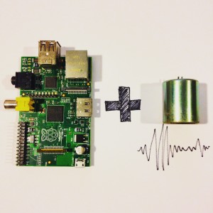
The seisMeowmeter is a project that used a geophone’s output to display realtime (or close to it) seismic data via an online graphing service, Plotly via a Raspberry Pi.

The seisMeowmeter project (AKA “Seismic Sundays” in the blog posts) was intended to be a more complete project with a full PCB created, firmware that performed more digital signal processing functions and a more elaborate radio link between the geophone and the RPi but other commitments at the time prevented the project from being fully complete. However, the seisMeowmeter will still be listed as a major project and its details are discussed here.

The live feed is intermittently operational and may be viewed here. If the live feed is down, the last few samples received will be shown.

The plots below show examples of the live feed and FFT of the seismic samples:

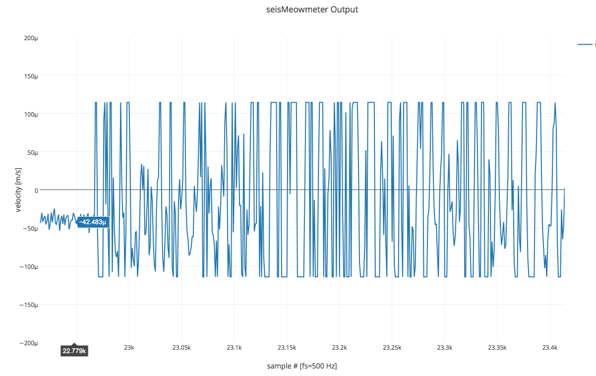
seismometer Live Feed Example

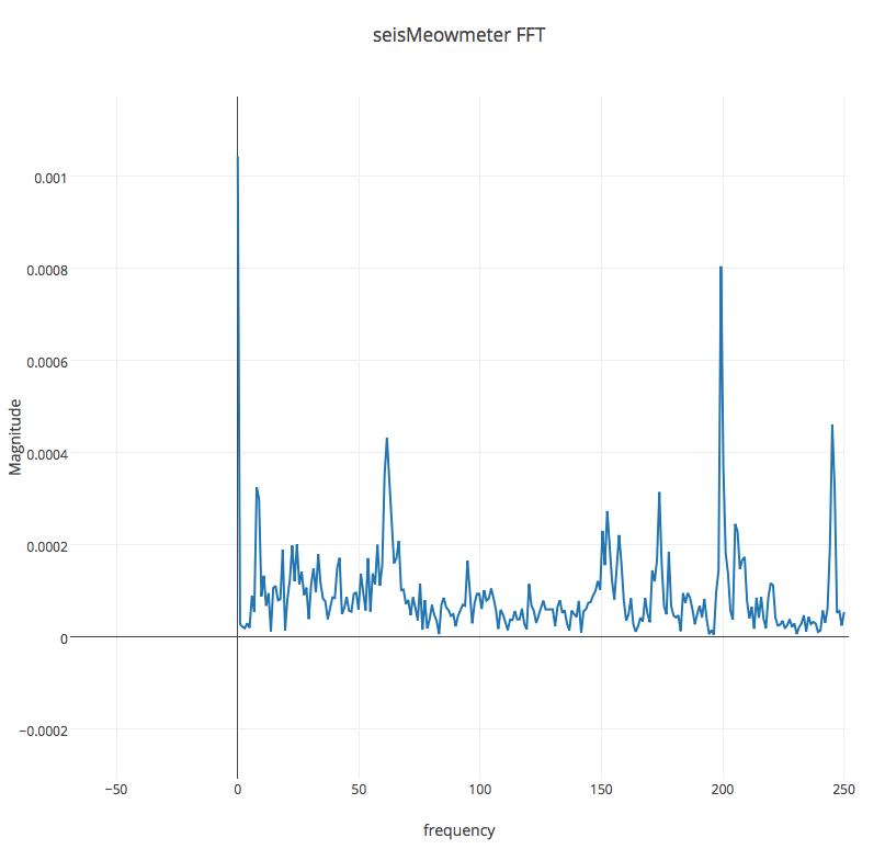
seisMeowmeter FFT Example

Overview

The object of the seisMeowmeter was simple. Create a seismology station which digitized the signals from a geophone, send the data over a radio link and the receiving end would do some additional signal processing and upload it to a server that would display the data in a real-time graph form. The planned block diagram looked like this:

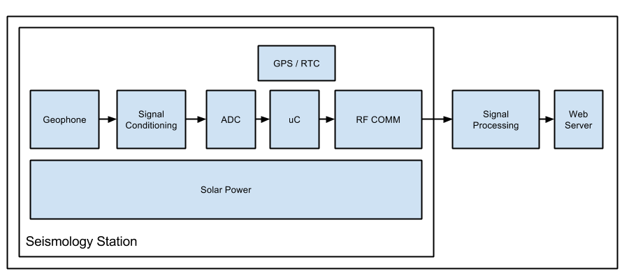
The geophone was to be attached to an analog front-end that would perform filtering and desired signal amplification which was then fed into an external, high resolution ADC (at least 12-bits, 24 if possible). A microcontroller would take in the ADC readings, possibly do some further processing to the signal and then send the data to the radio module. A GPS or RTC would time stamp the data as it went out into the airwaves. I wanted the station to have solar power as well to keep the station’s battery charged. Since I was not able to dedicate much of my time to the project, the design ended up looking more like this:

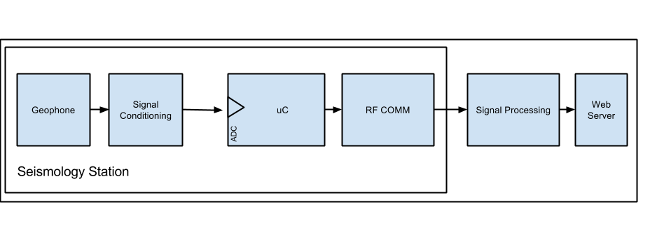
Instead of an external ADC, the microcontroller’s on-board ADC was used. Solar power and time stamping were removed and the radio used was a much smaller range off-the-shelf XBee unit. I used a Raspberry Pi along with Plotly’s APIs to receive the data stream and output the seismology data in graph form.

Hardware

Geophone

The geophone used was a SM-24 made by a company called Sensor. Relatively speaking, this geophone is low sensitivity and is more suited for reflective seismology (using a seismic wave source to create a profile of the geology of the area in study – much like SONAR for the ground) rather than for world seismologic studies which require instruments sensitive enough to detect seismic waves from the other end of the world.

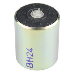
SM-24 Geophone (Image Credit: Sparkfun Electronics)

The geophone has a relatively flat frequency response between about 10 to 240 Hz and a resonant frequency at 10 Hz which will need to be dampened by a shunt resistance. The data sheet gives frequency plots with shunt resistances of 1 kΩ and 1.339 kΩ:

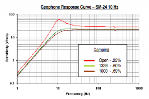
SM-24 Frequency Response (Image Credit: SM-24 Datasheet)

Analog Front End

Simply hooking up the geophone to a microcontroller isn’t quite enough. The output of a geophone is small and will need to be amplified and filtered to remove any stray high-frequency components that are not part of a seismic wave. This reference circuit was used to create a foundation upon which to build the front-end. The final circuit did not deviate much from the reference and had a few component value changes to tweak the frequency response to what I desired.

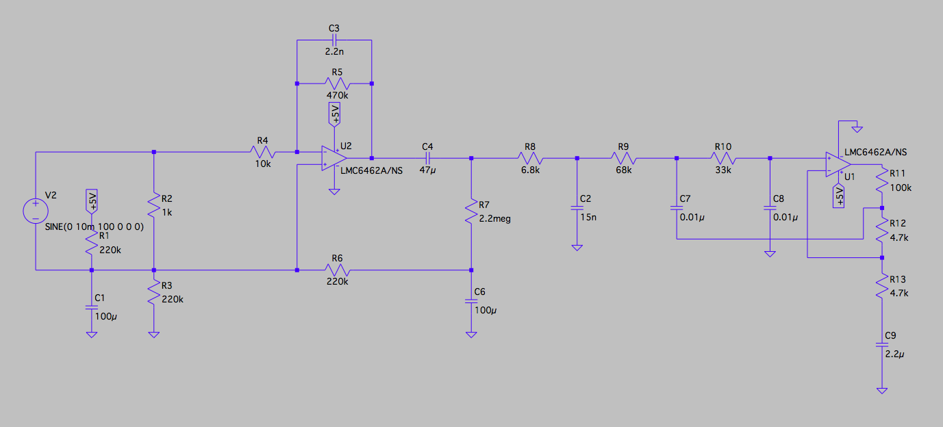
Final Analog Front-End Circuit

The circuit is simple. The geophone is connected to a 1 kΩ shunt resistor to dampen the ringing at 10 Hz. It then feeds into an amplifier with a gain of 47. It then goes through a cascading network of RC filters to create a low-pass filter with a cutoff frequency of about 100 Hz. The final op-amp stage serves two purposes. It further amplifies the signal by a factor of approximately 22 and it provides a positive feedback network to boost the cutoff frequency from about 100 Hz to about 250 Hz. The total gain of the system is about 1000 V/V. The op-amps used were the LMC6462, a nice low-power op-amp well-suited to this circuit. The output of the circuit is then fed into the ADC input of the micro controller with a bias of 1.65 V (as the rail voltage is 3.3 V)

Below are the simulated and actual plots of the conditioning circuitry:

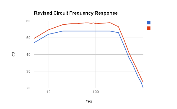
Red: Simulated Blue: Actual Circuit

Microcontroller

The conditioned geophone signal is fed into the ADC inputs of the Microchip dsPIC33FJ16GS502, a microcontroller (uC) built specifically for DSP purposes. The uC features a 10-bit ADC, which is not great but is good enough to show some waveforms for a proof of concept. The recommendations for ADC-specs for geophones are usually at least 24 bits. Originally, I planned on using the AD7714 by Analog Devices. The seismic data is sampled at the Nyquist rate of 500 Hz. The sampled data is then put into a buffer which is then sent out to the radio link via UART

Radio Link

Originally, I intended to use the TI CC1101 to transmit the seismic data to the Raspberry Pi. Instead, I used an XBee module which still did the trick. The seismic data is pulled from the buffer in the uC via UART at a baud rate of 57600. At the receiving end, another XBee is connected to the Raspberry Pi (via a USB adapter).

Firmware/Software

The firmware is relatively simple. A geophone sample is read at a rate of 500 Hz (the Nyquist rate) then placed into a ring buffer. A UART transmission routine runs in the background which upon complete transmission of the last sample, loads the next sample into the UART transmit register from the ring buffer.

At the Raspberry Pi end, a python script runs which queries the serial connection to the XBee for the sample data using the PySerial library. The data point is then uploaded to the Plotly streaming graph feed as well as added into a buffer which is then used to calculate the FFT of the cluster of samples. The FFT data is also uploaded to a Plotly graph but is not streaming.

The Future of the SeisMeowmeter

Unfortunately, the seisMeowmeter faced a stunted development. However, I hate to see it sitting sadly collecting dust on my workbench so I may be continuing its development. I would like to create a proper PCB with additional components (such as the external ADC) and perhaps a Bluetooth interface so that it can stream data to my iPad. It would be a good exercise on iOS development as well. Will the seisMeowmeter see new life? Time will tell…

Relevant Blog Posts

Seismic Sundays 0
Seismic Sundays 1
Seismic Sundays 2
Seismic Sundays 3
Seismic Sundays 4
Seismic Sundays 5
Seismic Sundays 6
Seismic Sundays 7