Time Domain FIR Filtering

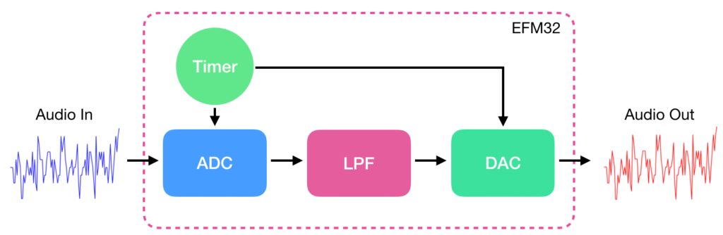
In the previous posts, we went through the basic exercise of reading audio samples through the ADC and outputting them to the DAC without manipulating the samples. This time, we’re going to kick things up a notch and add a filter to our audio processing chain.

Audio Sample with no Filtering

Audio Sample with Low Pass Filtering

Quick Review of FIR Filters

Below is a block diagram of a typical Finite Impulse Response (FIR) filter.

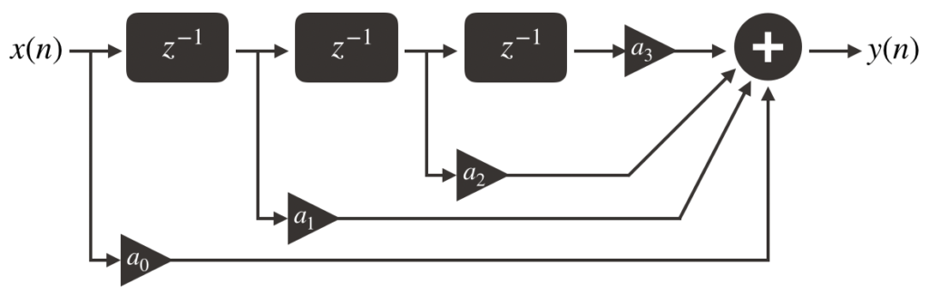
x(n) and y(n) represent the input and output (filtered) signals respectively. The blocks (z^-1) represent delay elements which store a sample and delay its propagation by one sampling period. An FIR can have any number of delay elements.

a0, a1, a2 and a3 are coefficients (also known as taps) which determine the filter’s cutoff frequency, cutoff slope and the type of filter (low pass, high pass etc). Typically, there are as many coefficients as there are delay elements + 1 (accounting for a0). However, this may not always be the case.

In operation, the network of delay elements shift out the value that they stored into the next delay element while storing new values shifted in by the previous delay elements. During each shift, a copy of the shifted values are scaled by the coefficients and then summed to obtain the output value.

As the coefficients play a crucial role in determining the filter behaviour, it is important to understand how to create them. We will start by creating a low pass filter.

Determining Coefficients

To create our low pass filter with cutoff frequency, fc, we need to figure out how to determine the correct coefficients. The method that we are using, called the window design method, is based on working with an ideal model of a filter to derive a practical one.

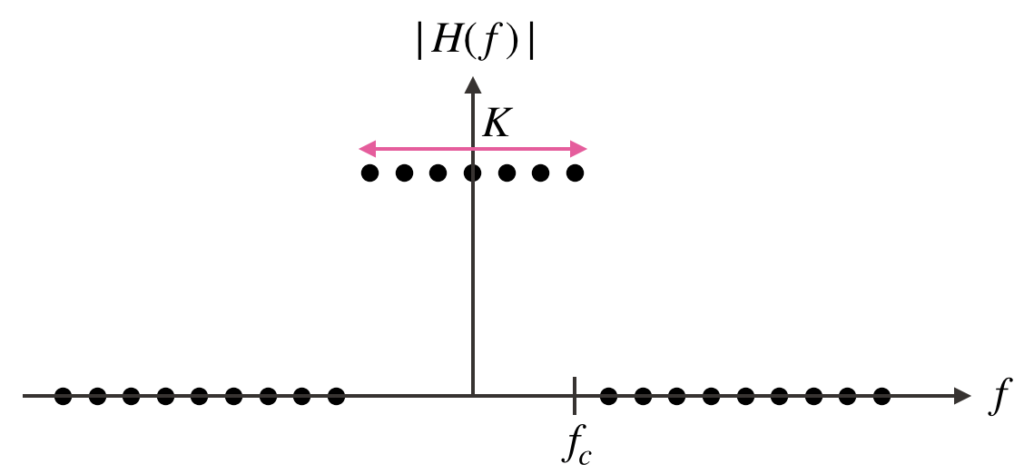
The above graph is an ideal representation of our FIR filter in the frequency domain. All frequencies past fc are blocked while those below are passed. Note that in practice, we often work with discrete systems hence, the representation of H(f) values as points rather than a continuous line.

To obtain the coefficients, we need to convert this frequency domain representation into its time domain representation. Applying the inverse Fourier transform yields the following equations:

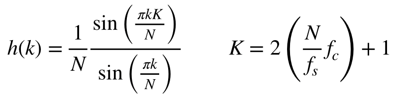
Where K is the passband width, N is the number of FFT points (eg. For a 1024-point DFT, N = 1024), fc is the cutoff frequency and fs is the sampling frequency. A plot of this equation is shown below:

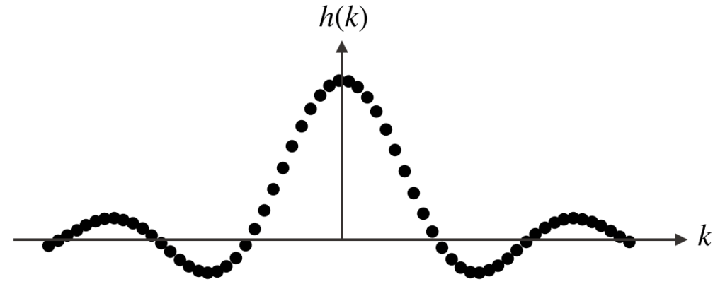
It turns out that h(k) represents the filter coefficients. While k, in theory, goes to +/- infinity, in terms of practicality only a handful of values can be used at the expense of filter ideality. Using more values will result in a more ideal filter response, but at the expense of more CPU resources.

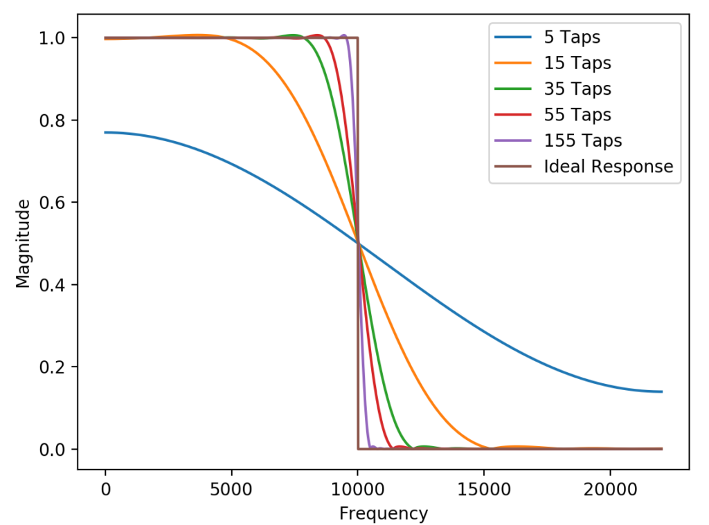
The above chart shows the performance of a low-pass filter with a cutoff frequency of 10 kHz. The more coefficients used, the closer the filter acts as an ideal filter.

When choosing coefficients, there is a catch. Suppose you choose to use 15 taps, then you will need to choose the values h(-7) to h(7) instead of h(0) to h(14). There is a symmetry required for expected FIR filter operation.

There are other design considerations to make – a big one being applying windowing to h(k) to minimize ringing artifacts that will occur as the number of coefficients applied to the filter increase. This is however beyond the scope of this post.

Implementation

While the ARM CMSIS DSP library does offer accelerated implementations of FIR filters, for now we’ll go through the longer route and manually implement the filter. While this approach is (very) inefficient, it serves the purpose of illustrating the concept.

Convolution

Once your coefficients are chosen and you have a buffer of audio samples ready for processing, applying the filter consists of a convolution operation mathematically described by the following equation:

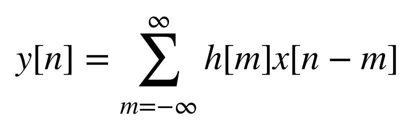
h refers to the filter coefficients. x refers to the buffer of audio samples and y is the filtered audio sample at some time, n. This operation can be thought of as a series of shift, multiply and adds – similar to the filter operation as described in Quick Review of FIR Filters.

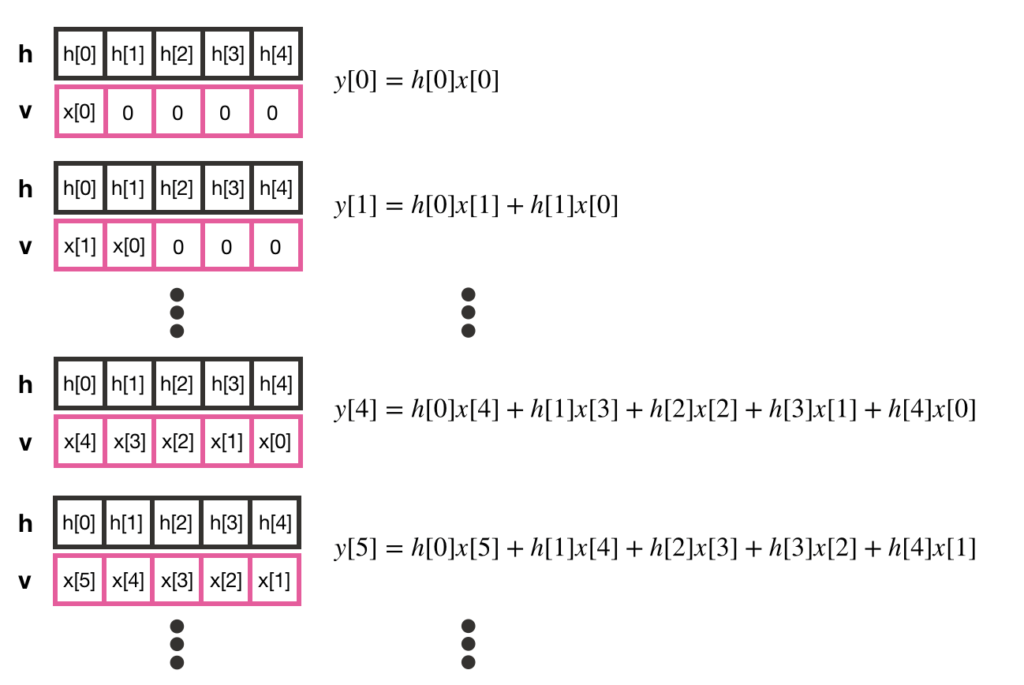
The above diagram illustrates the process of using convolution to calculate the filtered output for a given set of coefficients, h and audio samples, x. In this example, there are 5 filter coefficients h[n] stored in the array, h. The array v acts similarly to the delay elements (z^-1) in the FIR filter block diagram. v stores the audio samples, x[n] that get shifted in and out for each calculation of y[n]. The output, y[n] is calculated by multiplying each element in h with their corresponding elements in v and then summing the results. To calculate the next output sample, the last element in v is shifted out, a new audio sample is shifted in and the multiplication/add operation repeats.

Translating to Code

The following block of code implements the convolution process:

//  "Shift register" to hold audio samples for filtered output calculation
float32_t v[NUM_FILTER_COEFFS];

int filterAudioBlock(float32_t *x, size_t bufferSize, float32_t *h, size_t numFilterCoefficients, float32_t *y)
{
  //  Some safety checks
  if ((x == NULL) || (v == NULL) || (y == NULL))
    return -1;

  if ((bufferSize == 0) || (numFilterCoefficients == 0))
  {
    arm_fill_f32(0.f, y, bufferSize);
    return 0;
  }
  
  for (size_t i = 0; i < bufferSize; ++i)
  {
    //  Shift audio samples in v and add shift in new audio sample
    for (size_t j = numFilterCoefficients - 1; j > 1; --j)
      v[j] = v[j-1];

    v[0] = x[i];

    //  Multiply and add to get output value
    float32_t output = 0.f;
    for (size_t j = 0; j < numFilterCoefficients; ++j)
      output += h[j] * v[j];

    y[i] = output;
  }

  return 0;
}

This function takes as inputs, a buffer of audio samples, a set of filter coefficients and a destination to store the filtered audio samples. Each iteration of the outer loop shifts in a new sample of audio into the array, v. The first inner loop shifts shifts samples in v to their next position while the second inner loop carries out the multiply and add operations.

Creating Filter Coefficients

The following code uses the low-pass filter design equations in Quick Review of FIR Filters to calculate the filter coefficients:

int fir_calculateLPFCoefficients(float32_t fc, float32_t fs, const float32_t N, const uint32_t nTaps, float32_t *h)
{
  if ((h == NULL) ||(fs == 0) || (N == 0))
    return -1;
	
  if (nTaps % 2 == 0)
    return -1;
	
  float32_t passBandWidth = (2 * (N * fc / fs)) + 1;
	
  //  Since you can only use positive integers to index arrays, h[k=0] is shifted out to index (nTaps - 1) / 2 
  //  We calculate h(k=0) explicitly here to avoid the divide by zero issues
  h[(nTaps - 1) / 2] = passBandWidth / N;
	
  //  Calculate the first (nTaps - 1) / 2 coefficients on the positive k axis
  int hIndex = ((nTaps - 1) /2) + 1;
  for (int i = 1; i <= (nTaps - 1) / 2; ++i)
  {
    float32_t numerator = arm_sin_f32(PI * i * passBandWidth / N);
    float32_t denominator = arm_sin_f32(PI * i  / N);
		
    h[hIndex++] = (1 / N) * (numerator / denominator);	
  }
	
  //  Copy the calculated coefficients to the other half of the array to get the even symmetry
  for (int i = 0; i < (nTaps - 1) / 2; ++i)
    h[i] = h[nTaps - 1 - i];
	
  return 0;
}

There are a few key things to note here. First, we don’t need to calculate all nTaps coefficients. Due to the symmetry of h(k), we only need to calculate the (nTaps – 1) / 2 coefficients, then we can simply copy them to complete the coefficients array, h.

Second, since symmetry is expected about k=0, the total number of taps should be an odd number.

Finally, calculating the coefficient at k=0 will result in a divide by 0 error. However, since the limit of h(k) exists at this point, this value is explicitly calculated outside of the first for loop.

Putting it all Together

Using the framework built in the previous posts, this function can be used in the following manner:

// main.c
// ...

#define NUM_FILTER_COEFFS 9

const float32_t fs = 40000.f;
const float32_t fc = 500.f;
const float32_t N = 1024.f;

float32_t h[NUM_FILTER_COEFFS];
float32_t v[NUM_FITER_COEFFS];

int main(void)
{
  // ...

  int error = fir_calculateLPFCoefficients(fc, fs, N, NUM_FILTER_COEFFS, h);

  if (error)
    return error;

  while(1)
  {
    //  Check to make sure there is a buffer available for processing
    if (processingQueue[processingQueueHead] != NULL){

    //  Fancy processing code goes here
    //  In this case, our filtering function call
    error = filterAudioBlock(processingQueue[processingQueueHead], BUFFER_SIZE, h, NUM_FILTER_COEFFS, processingQueue[processingQueueHead]);

    if (error)
      //  Error handling

    transferBufferToQueue(processingQueue[processingQueueHead], dacQueue, &dacQueueTail);
    
    processingQueue[processingQueueHead] = NULL;
    processingQueueHead = (processingQueueHead + 1) % QUEUE_SIZE;

    }
  }
}

The filtering function is called in the infinite loop when there is a buffer of samples available in the processing queue. Once the filtered audio samples are calculated, they are transferred to the dacQueue.

Due to the nested loops in the function, filterAudioBlock(), the time complexity of the filtering operation is O(N^2). This means that as the number of filter coefficients go up, the number of computations increases exponentially. This creates a bigger risk of the actual processing time being greater than the allowed processing time causing irregularities in the audio.

For the hardware setup used here, for a buffer size of 512, the maximum number of filter coefficients usable before the system halts is 9. While there is a lot that can be done with a 40 MHz system, it does become rather limited very quickly!

In future posts, we will look at optimizing the filtering operation as well as implementing high and band-pass filters. An example project is also available on Github.

Further Reading

• The Scientist and Engineer’s Guide to DSP
• Introduction to Digital Filters by Julius O. Smith III