If you like math and haven’t yet seen 3blue1brown’s video on space-filling curves, I suggest you check it out.

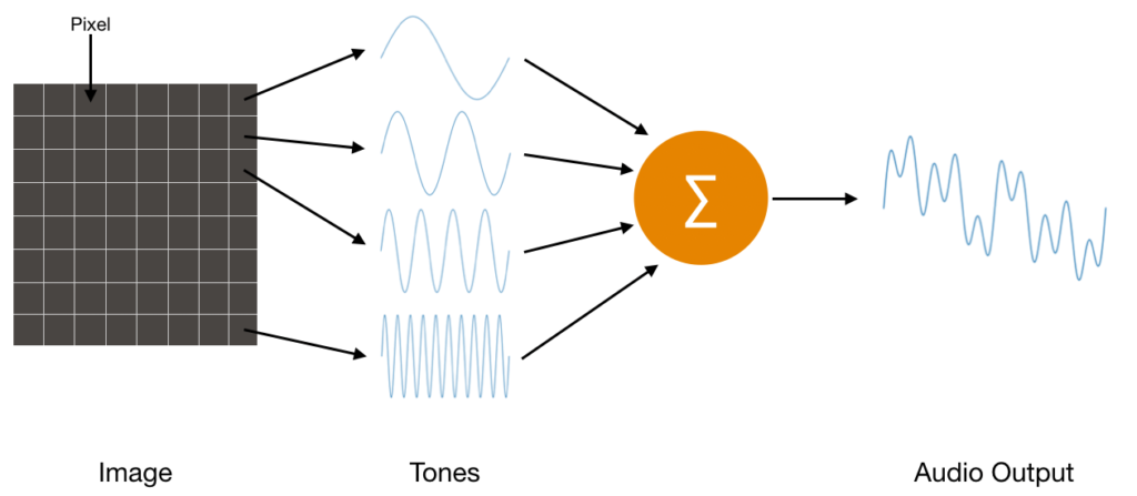
At the start of the video, a problem is given: provided an image, map each pixel to an audible frequency. The collection of unique frequencies of each pixel would then be summed, resulting in some waveform.

One approach is to draw a straight line from one pixel to the next one, eventually snaking your way to the last pixel. The resulting line represents a wound-up version of the frequency axis.

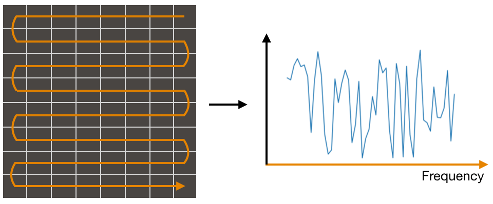
In this case, the top right pixel would represent the lowest frequency while the bottom right represents the highest frequency. The brightness (intensity) of each pixel determines the magnitude of its mapped frequency.

While this approach works, it does break down when your image’s pixel count increases AND you expect a pixel at some point, P to retain the same frequency mapping.

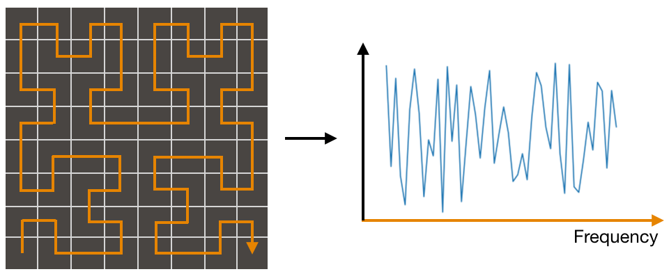
The video talks about an alternative approach where pseudo-Hilbert curves are used to map the pixels. The benefit to this approach is that when your image becomes larger, the mapping for point, P tends to converge to a particular frequency.

While the video was great in explaining Hilbert-curves, it didn’t quite give me a satisfying example of what an image “could” sound like so I decided to try it out and hear what I would get.

Using openFrameworks, I created a small application that would load in an image and calculate its frequency spectrum. This application would send the spectrum to a separate audio engine (written using JUCE) which would calculate the inverse FFT to give us the output time domain signal. The result was…interesting, if not a little underwhelming.

First Attempt

Here, we have a 128×128 pixel photo of a Pikachu doughnut. The pink curve below represents a partial view of the frequency spectrum (about 0 – 12 kHz). Anyone well versed in Fourier analysis is probably not surprised to hear the “clicking” sound coming out of their speakers.

Since just about every frequency bin has a relatively high magnitude, the resultant time domain signal approximates an impulse.

The number of frequency bins here is 16384. While this is equal to the total number of pixels (128 x 128 pixels), given the symmetric property of real number input FFTs, only half of the bins contain unique frequencies. This means that you cannot make a one to one relationship between a frequency bin and a pixel. You will need 32768 frequency bins to accomplish this. Instead, each frequency bin contains data from a block of M pixels. In this scenario, each frequency bin represents data from a block of 2 pixels.

The magnitude of each frequency bin is calculated by directly summing the scaled intensities of a pixel’s RGB channels.

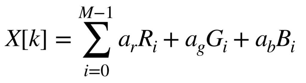
X[k] represents the magnitude at frequency bin, k. “a” represents the channel scaling factors while R, G and B are normalized pixel values. The summation occurs over a block of M pixels grouped to a specific frequency bin.

Maximum Pixel Gradient

While the above approach is one way to represent a scene via audio, it is difficult to discern any unique “features” of a scene when all you hear are relatively similar sounding clicks. This is especially true of an image that contains large uniform sections which would essentially create a flat frequency response characteristic of (sinc) impulses in the time domain.

In trying to reduce the influence of uniform sections, I decided to use the difference in intensity between neighbouring pixels to calculate the magnitude instead of using pixel intensities directly.

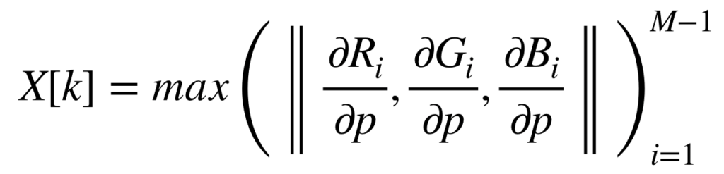
For a given block, the intensity of each pixel’s RGB channel is subtracted with the intensities of the previous pixel. The resulting delta R, G and B vectors are then used to calculate the Euclidean distance. This process iterates over all the pixels in the block with the final magnitude being the max difference found.

To further reduce the chance of obtaining a flat frequency response, the spectrum magnitude is “compressed” using a simple exponential function to further reduce weak magnitudes and exaggerate larger ones.

Here is the result:

While the audio is still a train of impulses, the timbre is closer to a “cymbal” than, say, the sound of a jackhammer. It’s hard to say if this is really any better than the previous approach but when testing with a webcam feed, movement was easy to discern as different frequencies faded in and out of hearing range.

The mapping methods in this post are certainly not the only ones worth trying. I have made the source code available on Github if you want to try out your own ideas. To build and run, you will need openFrameworks and JUCE. Do be careful to lower your speaker volume before running the code. You may get some unexpected and startling pop sounds as the time domain audio signal abruptly changes.